Backtest overfitting: how to detect it, with real cases

The problem

Overfitting is what happens when a model or a strategy learns the noise of the data it was chosen on. Picking the best of many backtests and judging it on the same history is the textbook case. The tools to detect it are well known: the deflated Sharpe ratio and the probability of backtest overfitting (Bailey and López de Prado 2014; Bailey, Borwein, López de Prado and Zhu 2016), the reality check and its successors (White 2000; Hansen 2005; Romano and Wolf 2005), false discovery rates (Benjamini and Hochberg 1995), and the warning that most published factors fail them (Harvey, Liu and Zhu 2016).

The harder part is using these tools without being fooled by them. Each one rests on assumptions about sample size, independence or the question asked, and we broke most of those assumptions at least once. The cases below come from our work on strategy evaluation for a funded-trader programme, where the judge is the share of simulated programmes that reach a profit target before a loss limit.

The probability of backtest overfitting needs many candidates

The probability of backtest overfitting (PBO) splits the history into blocks, picks the best configuration on half the blocks and checks where it ranks on the other half, over all splits. A PBO near 0 says the in-sample winner tends to stay good; near 0.5 says the choice was a coin toss.

In June 2026 an earlier version of our pipeline used a machine-learning router to cut the candidates down to five, then computed PBO on those five and got 0.467. The pipeline read that as “the selection is overfit” and returned a no-go. With five candidates, the out-of-sample rank of the winner can take only five values, and the median rank counts as a failure. The number is coarse and swings widely.

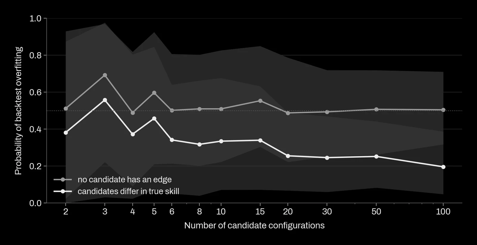
Line chart of PBO against number of candidates from 2 to 100, log scale. With no edge, PBO stays near 0.5 but jumps to 0.69 at 3 and 0.60 at 5. With real differences in skill, it falls from about 0.46 at 5 candidates to 0.20 at 100. Shaded bands are wide at small numbers. — Figure 1. Simulation. 1,000 daily returns per candidate, combinatorially symmetric cross-validation on 10 blocks (252 splits), 150 replications per point; bands are the 10th to 90th percentiles. Grey: no candidate has an edge. White: true daily means drawn with a spread of 0.03 standard deviations. With the same skill spread, PBO reads 0.46 at 5 candidates and 0.20 at 100, and at 5 candidates a single run can land anywhere from 0.07 to 0.85.

Two lessons came out of that episode. PBO is an indicator below about 100 candidates, never a gate. And it belongs to the population of candidates the search produced, not to a shortlist. Computed on the large population of survivors of the same search, it was between 0.00 and 0.07: the configurations were fine; the selection step was what had broken.

Deflate on the population, at the right N

A brute-force search over millions of configurations finds impressive backtests in pure noise: with 10⁶ to 10⁷ trials and no correction, the expected best Sharpe ratio is about 2.6 with no edge at all. One of our early runs left 71,000 configurations that passed every individual check. That was the signature of a missing deflation step, not of 71,000 edges. A sealed year then showed 19 of 20 of the top picks profitable, with inflated magnitudes.

The correction depends on how many tests you really ran, and correlated tests are not separate tests. In July 2026 we screened 14 options signals that were all variants of the level of volatility. A Bonferroni correction for 14 tests let nothing through. The effective number of tests, computed from the eigenvalues of their correlation matrix as (Σλ)²/Σλ², was 5.63. A false-discovery procedure kept 4 signals. The exact test was the null of the maximum: replay all 14 signals on a block bootstrap of the target (Politis and Romano 1994), keep the largest correlation of each draw, and compare the real maximum to the 95th percentile. That percentile was 0.0437; the real maximum, 0.0609, passed.

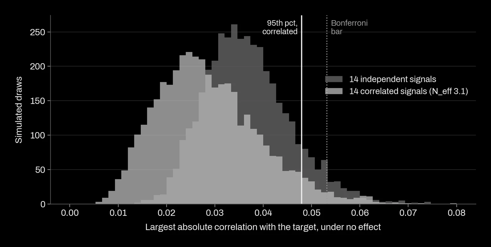
Two overlapping histograms of the largest absolute correlation under no effect: 14 independent signals centred near 0.035, 14 correlated signals centred near 0.027. The 95th percentile of the correlated case, 0.048, sits left of the Bonferroni bar at 0.053. — Figure 2. Simulation. A target of 3,000 observations with no effect, and 14 signals that are either independent or driven by three common factors (effective number 3.1), 4,000 draws. Under correlation the maximum is smaller, so the Bonferroni bar is too strict: pure noise crosses it 2.2 % of the time instead of the intended 5 %. The null of the maximum uses the 95th percentile of the correlated case directly.

Surviving the multiple-testing step was not the end. The surviving family then failed the split-half check (first half t = 0.68; the whole result came from the last two years), and its margin over simply holding the asset, 0.79 basis points a day, did not cover costs. Multiple testing comes first, then the stability checks, and neither replaces the other.

Why we do not tighten thresholds by the number of trials

The usual reflex is to raise the bar with every idea tried. We stopped doing that in 2026, for three reasons we measured.

First, it throws away real effects. Using the framework of Harvey and Liu (2020) to weigh missed discoveries against false ones, our old threshold of t = 3.31 discarded about 34 real effects for each false positive it avoided.

Second, the count of trials is an accounting artefact. It depends on how ideas are grouped and when the log was started; the amount of data does not. Wide searches make it worse: across 640 candidate pairs, the null of the maximum was +0.063, higher than the daily Sharpe ratio of the main strategy itself (0.0548). One grid of 456 cells produced a significance bar of 0.116 in information coefficient, above every effect in the literature. A wide sweep cannot decide anything; a bar raised to cover it would reject everything.

Third, a protection already exists that does not depend on the count. We develop freely and judge each candidate by its paired gain, a placebo and a planted effect at several sizes. Then one frozen candidate gets one read of a sealed sample, declared in advance. A single read has no multiplicity to correct. Evidence accumulates in a ledger of e-values, which stay valid under optional stopping (Ramdas, Grünwald, Vovk and Shafer 2023). We still report the number of trials with every verdict, as information. We use the null of the maximum or an effective N only when we have to pick one winner out of a population of configurations, which is the question those tools answer.

The stress signal that died twelve times

Over one night in July 2026 we tested about 52 new ideas for improving a deployed strategy, drawn from computer science, machine learning and quantitative finance. None survived. Several were stress precursors from very different fields: synchronisation of oscillators, change-point detection, self-exciting jump processes, the slope of an implied-volatility index. They really did predict the onset of stress, with lifts of 1.85 to 3.46 times the base rate. They added information the system did not have, and they passed their placebo and split-half checks.

Wired into the full system as a throttle or a veto, eight of them were judged and none added any pass rate. The reason was the same every time. The days that look stressed are also the days just before the sharp rebounds that pay for the strategy; cutting size on stress cuts the rebounds. The existing regime filter already captured the timing that mattered. The count has since reached twelve tests and twelve failures, and the rule is now a prior: a conditional lift measured outside the full chain never counts as evidence for the chain.

The heaviest attempt was a gradient-boosted regime model with fixed parameters, a walk-forward refit every 63 days with an embargo of 21 plus 2 days, 25 causal features and four variants. Its placebo was the same model trained on shuffled labels. The shuffled versions did as well as the real one: 0.63, the median of the noise. Its apparent skill was the mechanical effect of reducing size, not learning. An adversarial classifier told the eras apart with an AUC of 0.65: the features drifted between periods.

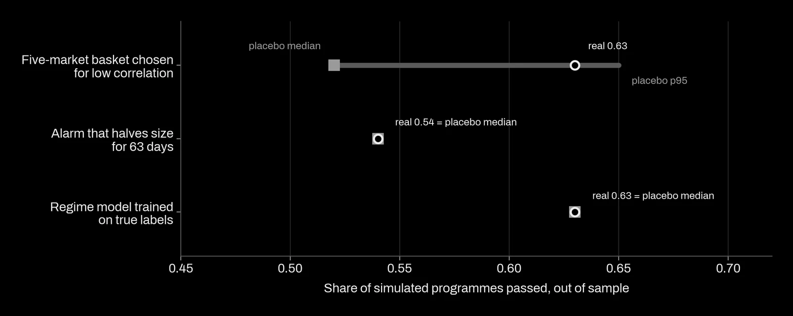
Dot chart of three items. Basket of five markets: real 0.63, placebo median 0.52, placebo 95th percentile 0.65. Alarm halving size: real 0.54 equal to placebo median. Regime model: real 0.63 equal to placebo median. — Figure 3. Real numbers, campaign of 17 July 2026, out-of-sample share of programmes passed. A five-market basket chosen for low correlation raised the pass rate from 0.54 to 0.63 (and ruin from 0.28 to 0.37); 30 random baskets reached 0.65 at their 95th percentile. A statistical alarm that halves size for 63 days did exactly as well as random alarms at the same frequency. The regime model equalled models trained on shuffled labels.

One variant looked like an escape: a precursor that timed a short position gave 0.89 with a ruin rate of 0.07 on its first run. Its threshold had been calibrated on a bull market with four signal days, so it had found eleven lucky days. With a causal threshold, the pass rate moved by -0.011, ruin by +0.016, and the placebo failed.

The Pareto wall in position sizing

When a programme ends on a profit target or a loss limit, position size decides two things at once: how fast the target comes and how often the limit is hit first. We tried about 25 sizing schemes, many borrowed from network congestion control, scheduling and optimal execution. At equal average aggressiveness, none beat the system's existing sizing (volatility-scaled, with the loss-reactive rule described below) in a stable way. Speed was bought with ruin at a near fixed rate. In the real system, a daily volatility of 1 % reached the target in about 159 days; 2 % in about 77 days, with a ruin rate of 0.35.

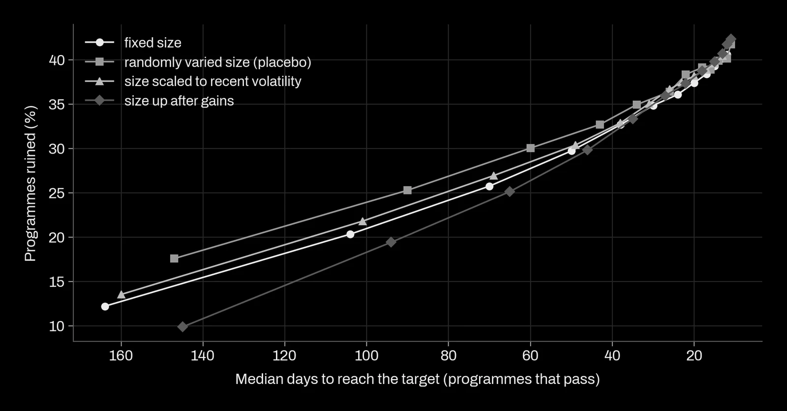
Line chart of ruin rate against median days to target for four sizing schemes at twelve levels of aggressiveness. All lie close to one rising curve; random size sits slightly above it, size up after gains slightly below it at the slow end. — Figure 4. Simulation. Daily returns with drift 0.05 % and fat tails (Student t, 4 degrees of freedom, 1 % volatility), target +10 %, loss limit -10 %, 500 days, 6,000 paths per point, size multipliers from 0.6 to 3.2. Fixed size goes from a 0.12 ruin rate in a median of 164 days to 0.39 in 15 days. Randomly varied size, our placebo, is worse at every speed. A rule that responds to the account's own gains and losses shifts the slow end a little; signal-driven rules sit on the line.

The wall taught us two controls. Every sizing test is run at equal average aggressiveness, and with a placebo where the signal that modulates size is permuted. Varying size near the barriers lowers ruin mechanically, with no predictive power at all; that artefact killed two candidates that had passed the aggressiveness check.

The one scheme that passed these controls was an additive-increase, multiplicative-decrease rule taken from network congestion control, which reacts to the account's own losses. Its headline gain of +0.2215 was not at equal aggressiveness, so we decomposed it: 93 % (+0.2062) came from the mechanism and 7 % from size. It traded 0.968 times smaller on average, and at equal size the variant without it was ruined 2.6 times as often (0.3108 against 0.1185).

Small numbers that lied

Some of the most expensive errors were single numbers.

Four numbers we trusted and what replaced them.
What we read	What it was	What we do now
A model that ranked strategy configurations scored 0.842 in tuning	Out-of-fold AUC 0.486, chance; the model was dropped in June 2026	Report only scores on folds the model never saw
No-edge baseline pass rate 0.37	0.269 when measured with the current engine	Measure the baseline with the judge itself, every time the judge changes
Sortino ratios near 10¹⁶ at the top of a ranking	Division by a downside deviation close to zero; capped in sample, uncapped out of sample	Never rank on a ratio whose denominator can vanish
PBO 0.467 on five configurations	A coarse statistic at small N	PBO only on the full population, as information

The baseline matters more than it looks. Every pass rate is read against what a strategy with no edge achieves under the same rules. With the baseline too high by 0.10, a real improvement can look like noise, and a mediocre one can look like a failure when it is not.

What this means for a project

When we build a model or select among options for you, you receive:

the number of variants we tried, reported with the result;
out-of-sample scores only, on folds or periods the model never touched, with a placebo that shows the score disappears when the information is destroyed;
any gain measured in the full system where it will run, rather than in isolation;
for any change of scale or risk, a comparison at equal aggressiveness, so that you do not pay for a gain with hidden risk.

What we refuse to claim: a winner picked and judged on the same data, a component that helps on its own but has not been tested inside your process, an overfitting score computed on a handful of candidates, or a ratio that can explode.

References

Bailey, D. H. and López de Prado, M. (2014). The deflated Sharpe ratio: correcting for selection bias, backtest overfitting and non-normality. The Journal of Portfolio Management 40(5). doi:10.3905/jpm.2014.40.5.094
Bailey, D. H., Borwein, J. M., López de Prado, M. and Zhu, Q. J. (2016). The probability of backtest overfitting. The Journal of Computational Finance. doi:10.21314/jcf.2016.322
White, H. (2000). A reality check for data snooping. Econometrica 68(5). doi:10.1111/1468-0262.00152
Hansen, P. R. (2005). A test for superior predictive ability. Journal of Business and Economic Statistics 23(4). doi:10.1198/073500105000000063
Romano, J. P. and Wolf, M. (2005). Stepwise multiple testing as formalized data snooping. Econometrica 73(4). doi:10.1111/j.1468-0262.2005.00615.x
Benjamini, Y. and Hochberg, Y. (1995). Controlling the false discovery rate: a practical and powerful approach to multiple testing. Journal of the Royal Statistical Society B 57(1). doi:10.1111/j.2517-6161.1995.tb02031.x
Harvey, C. R., Liu, Y. and Zhu, H. (2016). …and the cross-section of expected returns. The Review of Financial Studies 29(1). doi:10.1093/rfs/hhv059
Harvey, C. R. and Liu, Y. (2020). False (and missed) discoveries in financial economics. The Journal of Finance 75(5). doi:10.1111/jofi.12951
Politis, D. N. and Romano, J. P. (1994). The stationary bootstrap. Journal of the American Statistical Association 89(428). doi:10.1080/01621459.1994.10476870
Ramdas, A., Grünwald, P., Vovk, V. and Shafer, G. (2023). Game-theoretic statistics and safe anytime-valid inference. Statistical Science 38(4). doi:10.1214/23-STS894

Detecting backtest overfitting