

The question: how do you split data in time?
Cross-validation estimates how well a model will do on data it has not seen. The textbook version cuts the rows into k random folds, trains on k − 1 and tests on the last. That works when rows are independent. In a time series they are not: today's features look like yesterday's, and a target defined over the next 20 days shares 19 of its days with yesterday's target. A random split puts those near-copies on both sides of the line, and the model is graded on questions it has already seen the answer to.
This note is only about how to split. Two neighbouring problems have their own notes: data that was not known on the day it is used (point-in-time data, revisions, publication delays) in how we treat data, and the inflation that comes from trying many models in detecting overfitting. A perfect split does not repair either.
Rather than argue, we measured. We built a series where we know the true out-of-sample skill of each model, then asked five splitting schemes to estimate it.
The experiment
Each history is 2,000 daily returns. A hidden state drifts slowly (an autoregressive process with persistence 0.98), and each day's return is a small multiple β of yesterday's state plus noise. The model sees five features, all computed from data up to the day itself: the mean return of the last 5, 20 and 60 days, the volatility of the last 20 days, and a noisy reading of the hidden state. The target is the sum of the next 20 returns, so consecutive targets overlap by 19 days, as in most forecasting and trading labels.
We ran two worlds. In the first, β = 0: the future is pure noise and any honest estimate should be at or below zero. In the second, β = 0.2: there is a small real signal. For each world we simulated 30 independent histories and fitted two models: a random forest (100 trees, at least 5 rows per leaf) and a ridge regression. The true skill of a history is the R² of the model fitted on all 2,000 days and scored on 6,000 fresh days of the same process. A real dataset cannot give that number, which is why we used a simulation.
The true R² of the forest in the noise world is −0.17, not zero. A flexible model fitted to noise predicts noise, and its predictions add error to the plain mean. That is the number a correct method should find.
Five ways to split
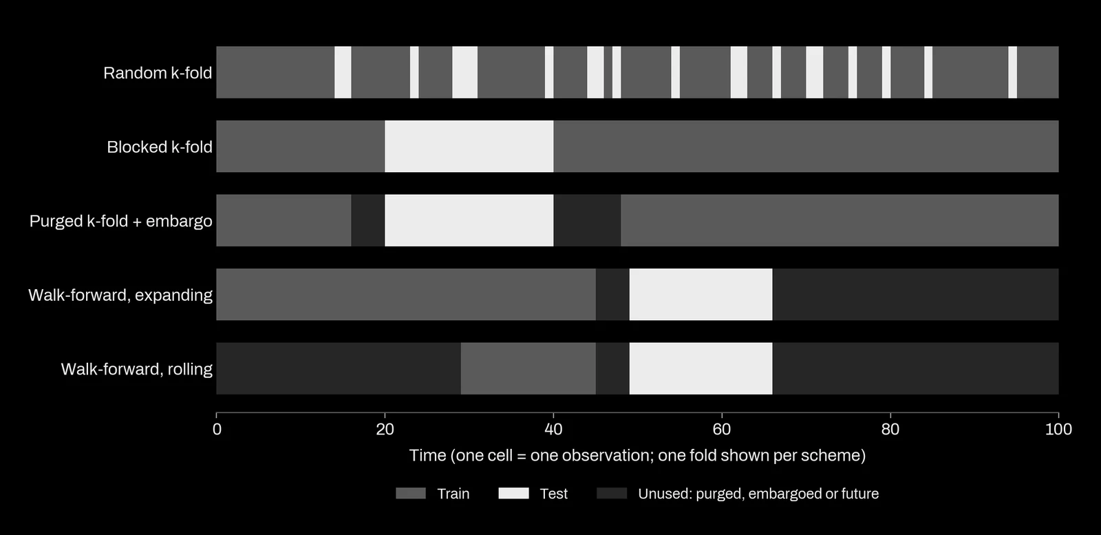
- Random k-fold. Rows shuffled into 5 folds. The default in most libraries.
- Blocked k-fold. 5 contiguous blocks of 400 days, each tested once, the model trained on the rest, past and future.
- Purged k-fold with an embargo. Blocked, but every training row whose 20-day label window overlaps the test labels is removed on both sides of the block (the purge), and a further 20 days after the block are dropped (the embargo), because their trailing features read returns from inside the test period. The idea goes back to the h-block cross-validation of Burman, Chow and Nolan (1994) and Racine's hv-block (2000); the purge and embargo names come from López de Prado (2018).
- Walk-forward, expanding. The series is cut at five dates; each test block is predicted by a model trained on everything before it, with a 20-day gap so that no training label reaches into the test period. The first model sees 333 days, the last 1,647.
- Walk-forward, rolling. The same, with the training window fixed at the most recent 333 days.
The gap in walk-forward is the point most often forgotten. Without it, the last training label covers the first 19 days of the test block, and walk-forward leaks too.
What each scheme reported
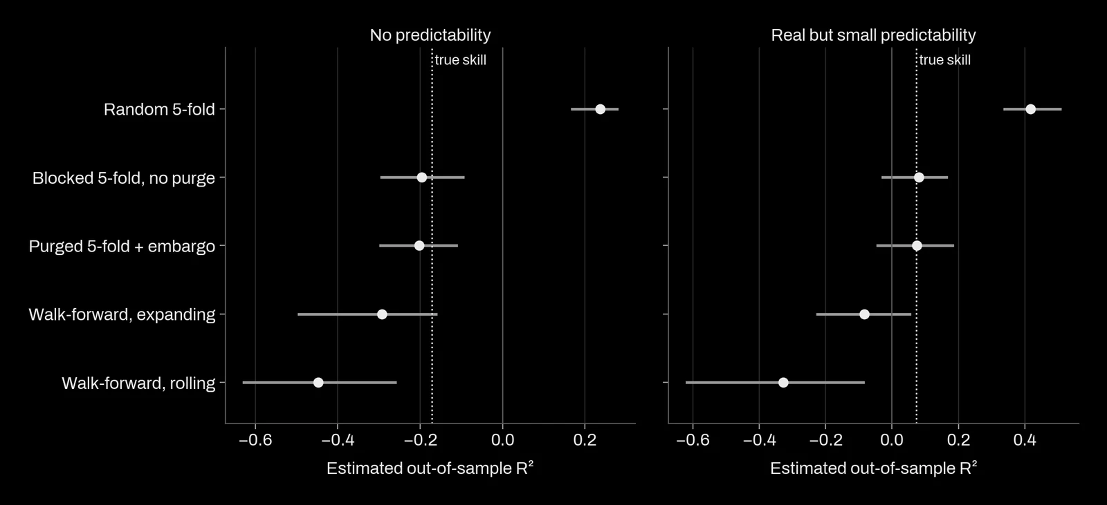
| World, model | True | Random | Blocked | Purged + embargo | Expanding | Rolling |
|---|---|---|---|---|---|---|
| Noise, forest | −0.171 | +0.236 | −0.196 | −0.202 | −0.292 | −0.447 |
| Noise, ridge | −0.048 | +0.025 | −0.049 | −0.052 | −0.183 | −0.447 |
| Signal, forest | +0.073 | +0.417 | +0.081 | +0.074 | −0.084 | −0.328 |
| Signal, ridge | +0.199 | +0.259 | +0.206 | +0.203 | +0.108 | −0.154 |
Random k-fold overstates skill, and by a lot for a flexible model. On pure noise it reported a positive R² for the forest in 30 histories out of 30, on average +0.236 where the truth was −0.171: an optimism of 0.41. With a real signal it reported +0.417 for a true +0.073, more than five times the real value. The mechanism is simple. For a test day, the training set holds the day before and the day after, whose features are almost identical and whose targets share 19 of 20 returns. A forest with small leaves finds that neighbour and copies its answer.
A linear model leaks much less. Ridge regression cannot memorise neighbours, so its optimism under random k-fold was 0.073 in the noise world and 0.060 with the signal. Bergmeir, Hyndman and Koo (2018) showed that ordinary k-fold is valid for purely autoregressive models whose errors are uncorrelated. Overlapping targets break that condition, so a small leak remains, but the size of the damage depends on the model. This matters in practice: when someone compares a linear baseline to a boosted model with random k-fold, the comparison is biased in favour of the more flexible model.
Purged k-fold with an embargo found the truth. In the signal world it estimated +0.0745 for a true +0.0734; for ridge, +0.203 for +0.199. In the noise world it was slightly pessimistic (−0.202 against −0.171), because each fold trains on 1,600 days or fewer instead of 2,000. Plain blocked k-fold was almost as good here; the next section shows when it is not.
Walk-forward was honest about time but pessimistic and noisy. The expanding scheme estimated −0.084 for a true +0.073, and only 17 % of histories gave a positive estimate for a model that does have skill. Its folds train on 333 to 1,647 days, so it measures a model trained on less data than the one that will be deployed, and its spread across histories (standard deviation 0.143) was larger than that of the purged scheme (0.089). The rolling window, fixed at 333 days, was worse still.
When the purge matters
Two quantities drive the leak: how far the label looks ahead, and how short the test blocks are compared with that horizon.
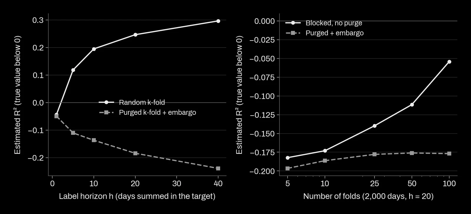
With a one-day target there is no overlap, and random k-fold gave −0.044 against −0.050 for the purged scheme: the leak through autocorrelated features alone was small for this process. At a 5-day horizon random k-fold already reported +0.118, at 20 days +0.247, at 40 days +0.297, while the purged scheme stayed between −0.110 and −0.239. The longer the label, the bigger the lie.
With the horizon fixed at 20 days, plain blocked k-fold without a purge looks safe with 5 folds (−0.182, against −0.197 with purge and embargo, on six fresh histories). It stops being safe as the blocks shrink: with 25 folds of 80 days it reported −0.140, with 50 folds −0.112, and with 100 folds of 20 days −0.054, while the purged version stayed between −0.176 and −0.197 at every fold count. Each test block leaks through its two edges, so the leak grows with the number of edges. Leave-one-out and many-fold schemes, often chosen to squeeze a short history, are where an unpurged split does the most damage.
How we choose a scheme
The simulation is stationary: the rule linking features to the future never changes. Real series are not, and that changes the trade-off. Cerqueira, Torgo and Mozetič (2020) compared estimation methods on 62 real series and on synthetic ones: cross-validation variants did well on stationary series, while on real series with non-stationary variation the most accurate estimates came from out-of-sample methods that keep the time order. Our rules follow from both results.
- Never random k-fold when rows are close in time, unless the target is one step ahead, the model is linear and a check like the one above shows the leak is negligible.
- Purge at least the label horizon on both sides of every test block, and add an embargo at least as long as the horizon after it. If a feature reads further back than the label reads forward, we embargo the longer of the two.
- Use purged k-fold to compare and tune models when the history is short and the process looks stable: it uses all the data and its estimates are less noisy.
- Use walk-forward to estimate the level a deployed model will reach, because deployment is walk-forward: the model is retrained on the past and meets a future that may differ. Report each fold separately, since a drift shows as a trend across folds, which an average hides.
- Keep a final block at the end, sealed, read once after every choice. Our gates note explains why one read and not two.
- Put every fitted step inside the folds: scaling, feature selection, imputation and hyperparameter search. A scaler fitted on the full series has seen the test period. A tuning loop needs its own inner split that follows the same rules (nested cross-validation).
- Split panels by time, not by entity. With many series (shops, sensors, assets), a random split of entities leaves the same dates on both sides, and a market-wide shock is learned in training and tested on the same day.
Two cheaper options exist and we use them when they fit. Sampling one row every h days removes the label overlap at the cost of most of the data. And a placebo, the same pipeline run on a target shifted so that it cannot be predicted, should score at or below zero under the chosen split; if it scores above, the split leaks.
The reviews by Arlot and Celisse (2010) for cross-validation in general, Roberts and co-authors (2017) for dependent data in ecology and Tashman (2000) for forecasting evaluation are good starting points; Bergmeir and Benítez (2012) gave one of the first systematic comparisons for time series predictors.
What this means for a project
On a forecasting or time series project with us, you receive:
- a written split design before any model: label horizon, purge and embargo widths, fold boundaries, the final sealed block and why each was chosen;
- model comparisons on purged folds, paired on the same folds, with fold-level results and not only an average;
- a walk-forward replay that retrains the model as it would be retrained in production, giving the level to expect and its trend across time;
- a leak check: the same pipeline on a placebo target, and the gap between random and purged splits, so you can see how much a naive split would have flattered the model;
- the code of the splitter, with tests that fail if a training label overlaps a test label.
What we refuse to report: a random k-fold score for a model trained on overlapping targets, or a walk-forward score without a gap. The simulation behind this page is kept with the site sources and reruns with the same seeds.
References
- Bergmeir, C. and Benítez, J. M. (2012). On the use of cross-validation for time series predictor evaluation. Information Sciences 191. doi:10.1016/j.ins.2011.12.028
- Bergmeir, C., Hyndman, R. J. and Koo, B. (2018). A note on the validity of cross-validation for evaluating autoregressive time series prediction. Computational Statistics and Data Analysis 120. doi:10.1016/j.csda.2017.11.003
- Cerqueira, V., Torgo, L. and Mozetič, I. (2020). Evaluating time series forecasting models: an empirical study on performance estimation methods. Machine Learning 109. doi:10.1007/s10994-020-05910-7
- Tashman, L. J. (2000). Out-of-sample tests of forecasting accuracy: an analysis and review. International Journal of Forecasting 16(4). doi:10.1016/S0169-2070(00)00065-0
- Arlot, S. and Celisse, A. (2010). A survey of cross-validation procedures for model selection. Statistics Surveys 4. doi:10.1214/09-SS054
- Burman, P., Chow, E. and Nolan, D. (1994). A cross-validatory method for dependent data. Biometrika 81(2). doi:10.1093/biomet/81.2.351
- Racine, J. (2000). Consistent cross-validatory model-selection for dependent data: hv-block cross-validation. Journal of Econometrics 99(1). doi:10.1016/S0304-4076(00)00030-0
- Roberts, D. R. et al. (2017). Cross-validation strategies for data with temporal, spatial, hierarchical, or phylogenetic structure. Ecography 40(8). doi:10.1111/ecog.02881
- López de Prado, M. (2018). Advances in Financial Machine Learning. Wiley, chapter 7 (purged and embargoed cross-validation). OpenAlex W2968584812.