

Why intermittent demand needs its own methods
A spare part, a slow catalogue item or a hospital consumable is often not sold at all in a given month, then sold three at once. Most months are zero, the sizes vary, and the useful question is rarely the next month's figure. It is how much stock covers the lead time with a given probability. Methods built for smooth sales behave badly here. Exponential smoothing drops after every zero and jumps after every sale, so its forecast is highest just after a demand, which is when the next one is least likely.
Croston's method was the first answer. It splits the series into two parts: the size of each non-zero demand and the interval between two demands, smooths both separately, and forecasts their ratio. Both are updated only when a demand occurs. Syntetos and Boylan later showed that this ratio is biased upward and proposed multiplying it by (1 − α/2), where α is the smoothing constant; that is the SBA method. Teunter, Syntetos and Babai (TSB) changed the second part: instead of the interval, they smooth the probability that a demand occurs, and update it every period. When demand stops, the TSB forecast decays towards zero, while Croston and SBA keep the last level for as long as no sale arrives. That matters for parts that become obsolete.
We wanted numbers rather than the usual verbal ranking, on data anyone can download, with a protocol strict enough that the result would carry over to a real catalogue. This note is about the methods and the measurement. Our demand planning work for clients is described on the forecasting service page.
Data and protocol
We used the car parts data from Hyndman, Koehler, Ord and Snyder (2008): 2,674 monthly series of sales of car parts, January 1998 to March 2002, 51 months each, distributed with the R package expsmooth on CRAN. We dropped the 165 series with missing months and the 105 series with fewer than two demands in the first 39 months, since no method can be fitted or scaled on them. That leaves 2,404 series, in which 74.0 % of all months are zero.
Every setting was chosen on a development window and then frozen:
- Development: fit on months 1 to 39, forecast months 40 to 45. We chose the moving-average window (3, 6, 12 or 24 months), the smoothing constants (0.05, 0.1, 0.2 or 0.3) and the loss of the boosting model on this window, by mean RMSSE.
- Sealed: fit on months 1 to 45, forecast months 46 to 51 (October 2001 to March 2002) at horizons 1 to 6, read once.
The development window picked a 12-month moving average, α = 0.1 for simple exponential smoothing (SES), α = 0.3 for Croston and for SBA, and α = 0.3 for sizes with β = 0.1 for the probability in TSB. Three of these sit at the top of the grid, a first sign that the series were moving. The pooled model is a single gradient-boosting model (LightGBM) trained on all series at once, one row per series, forecast origin and horizon. Its inputs are the last 12 months, rolling means over 3, 6, 12 months and the whole history, the share of non-zero months, the months since the last demand, the horizon and the calendar month, all divided by the series' own mean so that series of different sizes can share one model. On the development window a Tweedie loss gave a mean RMSSE of 0.695 and squared error 0.700, so we kept Tweedie.
We also forecast zero for every series and every month. It is not a method anyone would deploy, and that is the point: a metric that ranks it first is telling you something about the metric.
Classifying the series: ADI and CV²
Syntetos, Boylan and Croston (2005) proposed classifying each series by two numbers. The ADI (average demand interval) is the average number of periods between two demands. The CV² is the squared coefficient of variation of the non-zero demand sizes. They derived cut-offs of 1.32 for ADI and 0.49 for CV² from the regions where SES or SBA has the lower theoretical error, which gives four classes: smooth (frequent, regular sizes), erratic (frequent, variable sizes), intermittent (rare, regular sizes) and lumpy (rare, variable sizes).
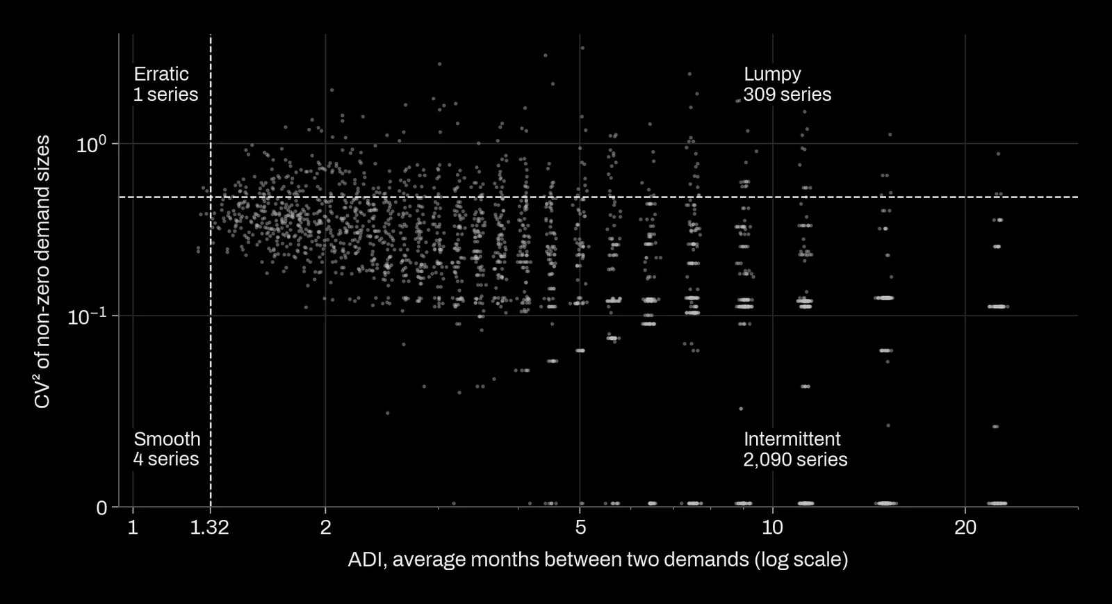
On this data the scheme puts 2,090 series in the intermittent class and 309 in the lumpy class. Only 5 series are smooth or erratic, too few to say anything about, so the results below are given for all series, intermittent and lumpy. The classification is a starting point for choosing a method, not a substitute for testing one: as the next sections show, the method the scheme recommends was not the most accurate here.
Choosing the metric before the method
MAPE cannot be used. It divides each error by the actual value, and the actual value is zero in 79.3 % of the sealed months; 99.1 % of the series have at least one zero month in the window. Dropping zero months does not fix it: what remains is an error measured only on the months with a sale, which rewards forecasts that are too high. Symmetric variants that divide by the sum of forecast and actual give the maximum error to every month where one of the two is zero, whatever the size of the miss.
The usual replacements are scaled errors. MASE (Hyndman and Koehler, 2006) divides the mean absolute error by the mean absolute change of the series from one month to the next in the fitting period. RMSSE, used to rank the M5 competition, does the same with squared errors. Both are free of units, so they can be averaged across parts that sell 1 or 100 a month, and both are finite when actual values are zero.
They do not reward the same forecast. Absolute error is minimised by the median of the future demand, and squared error by its mean (Kolassa, 2020). When more than half the months are zero, the median is zero. A forecast of zero then scores well on MASE, and it did: it had the lowest MASE of all eight forecasts on 85.7 % of the series, and the lowest mean MASE, 0.625, against 0.872 for the next best. A forecast of zero orders nothing. We report MASE because readers expect it, but we never rank intermittent forecasts on it.
RMSSE targets the mean, which is what a stock calculation needs. On this window, though, the zero forecast also had the lowest RMSSE (0.526, against 0.557 for the 12-month moving average). The reason is in the data, shown on the left of Figure 2: the mean demand per series and month fell from 0.643 in 1998 to 0.389 in the sealed window, and the share of months with a sale from 27.3 % to 20.7 %. Every method that learns a level from the past over-forecast. A falling catalogue makes doing nothing look good on any point metric.
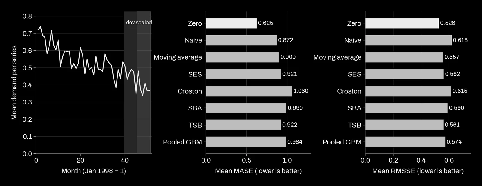
So we read three numbers together: RMSSE for accuracy of the level, the bias (mean forecast over mean actual) because stock is bought on the level, and a quantile loss for the service level. None of them alone picks a sensible method.
What won, and by how much
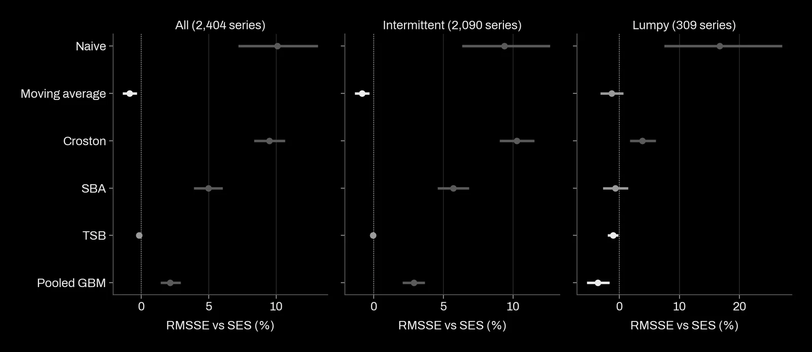
Differences between methods were measured series by series: for each pair we took the difference in RMSSE on every series, then resampled the series 4,000 times to get a 95 % interval on the mean difference. Pairing matters because the series differ far more from each other than the methods do.
| Method | Mean RMSSE | Against SES, all series | Against SES, lumpy (309) | Bias |
|---|---|---|---|---|
| Zero | 0.526 | -6.4 % [-8.1; -4.7] | -5.8 % [-11.7; -0.1] | -100 % |
| Moving average, 12 months | 0.557 | -0.9 % [-1.4; -0.3] | -1.3 % [-3.2; +0.7] | +18 % |
| TSB | 0.561 | -0.2 % [-0.3; +0.0] | -1.1 % [-1.9; -0.2] | +21 % |
| SES | 0.562 | reference | reference | +23 % |
| Pooled boosting | 0.574 | +2.1 % [+1.4; +2.9] | -3.6 % [-5.4; -1.7] | +6 % |
| SBA | 0.590 | +5.0 % [+3.9; +6.0] | -0.7 % [-2.8; +1.4] | +16 % |
| Croston | 0.615 | +9.5 % [+8.4; +10.6] | +3.8 % [+1.7; +6.1] | +37 % |
| Naive (last month) | 0.618 | +10.1 % [+7.2; +13.1] | +16.7 % [+7.4; +27.1] | -10 % |
Five findings, in order of how firmly we hold them.
- SBA beats Croston. Same structure, one correction factor: RMSSE 0.590 against 0.615, bias +16 % against +37 %. The upward bias that Syntetos and Boylan derived is visible in real data. There is no reason to run plain Croston.
- Among the classical methods, the plain ones held. The 12-month moving average, TSB and SES finished within 1 % of each other, ahead of SBA by 5 % on all series and by 5.7 % on the intermittent class, where the classification would have recommended SBA. On a declining catalogue a method that keeps its level until the next sale is slow to follow the decline; TSB, which lowers its probability every month without a sale, was built for this and was never measurably worse than SES.
- The pooled model was the least biased. It over-forecast by 6 %, where every single-series method was between +16 % and +37 %. Trained across all series, it learned that parts in this catalogue tend to fade. Its RMSSE was 2.1 % worse than SES overall but 3.6 % better on lumpy series, the best of any real method in that class.
- The gaps are small. Apart from naive and Croston, every method is within 5 % of SES. On intermittent data the noise in a single month dominates the error, and no point forecast removes it. That is why the quantile matters more than the point.
- The zero forecast won on RMSSE because demand fell. We read it as a warning about this window, not as advice.
Service level: the 90 % quantile
Stock is set from a quantile. If we want a 90 % chance that one month of demand is covered, we need the 90th percentile of next month's demand, not its mean. We compared four ways of getting it:
- a Poisson distribution with the SBA forecast as its mean;
- a negative binomial with the SBA forecast as its mean and a variance estimated from SBA's own one-step errors over months 25 to 45;
- the empirical 90th percentile of the last 24 months;
- the pooled boosting model trained directly on the quantile (pinball) loss at 0.9.
We scored them by coverage (the share of sealed months at or below the quantile) and by the pinball loss divided by the same scale as MASE (Kolassa, 2016, discusses why count forecasts should be judged as distributions).
| Quantile forecast | Coverage | Scaled pinball loss |
|---|---|---|
| Poisson around SBA | 93.8 % | 0.417 |
| Negative binomial around SBA | 93.8 % | 0.429 |
| Empirical, last 24 months | 95.4 % | 0.366 |
| Pooled boosting, quantile loss | 91.7 % | 0.374 |
The empirical quantile beat the Poisson quantile by 12.2 % on pinball loss (interval -15.5 % to -9.2 %). The negative binomial, which should handle the extra variance, was 3.1 % worse than the Poisson (+1.3 % to +5.0 %), probably because its variance was estimated over months when demand was higher. The boosting model came closest to the 90 % target, at 91.7 %, but its pinball loss was not distinguishable from the empirical quantile: +2.2 %, interval -0.8 % to +5.1 %.
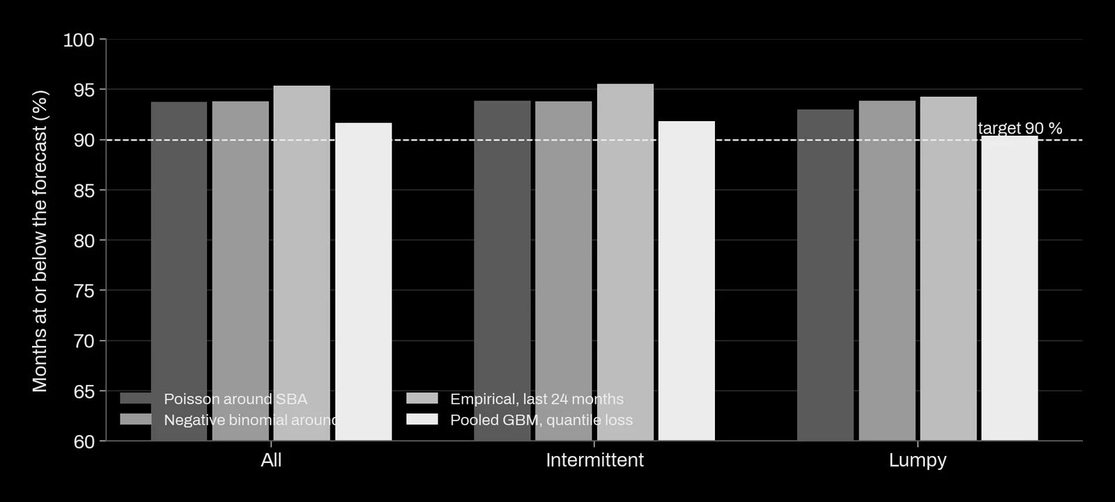
Coverage on counts is coarse. A quantile of 0 covers every month without a sale, which here is 79.3 % of them, so coverage near 90 % is easy to reach and says little by itself. The pinball loss is what separates the methods: it charges 0.9 per unit of unmet demand and 0.1 per unit of excess stock, which is a stock policy written as a metric.
How to run this on your own catalogue
- Count zero months and compute ADI and CV² per item. If most items are intermittent or lumpy, drop MAPE from every report before anything else.
- Include a zero forecast, a naive forecast and a moving average in the comparison. If a method does not beat the moving average on RMSSE, it is not earning its complexity.
- Choose smoothing constants and model settings on one window, then score once on a later window that no choice has touched.
- Report RMSSE, bias and a scaled pinball loss at the service level you actually target, with paired intervals across items, overall and per class.
- Plot the mean demand per item over time. If the catalogue is declining or growing, say so next to the results: the ranking will depend on it.
- Prefer SBA to Croston, and TSB when items can become obsolete. Try a pooled model when you have hundreds of items or more: its gain here was on bias and on lumpy items, not on average accuracy.
Limits of this study: one public dataset, from 1998 to 2002, with a single sealed window of six months and a declining catalogue. Lead times, order costs and the link from forecast to stock level were not modelled. The boosting model was tuned only on its loss function. A different catalogue can rank the methods differently, which is why we rerun the comparison on each client's data rather than reuse this table.
What this means for a project
On a demand forecasting project for slow-moving or spare-part items, you receive:
- a profile of your catalogue: share of zero months, ADI and CV² per item, and the trend of demand over time;
- a benchmark on your history with zero, naive, moving average, SES, SBA, TSB and a pooled model, scored on a window held back until the end, with paired intervals;
- accuracy, bias and a quantile loss at your service level, overall and per class, never MAPE on intermittent items;
- quantile forecasts per item that feed your reorder points, with their measured coverage.
What we will not do: rank methods on a metric a forecast of zero can win, recommend a method because the classification says so without testing it on your data, or report one accuracy figure for a catalogue whose demand is drifting.
References
- Croston, J. D. (1972). Forecasting and stock control for intermittent demands. Operational Research Quarterly 23(3). doi:10.1057/jors.1972.50
- Syntetos, A. A. and Boylan, J. E. (2005). The accuracy of intermittent demand estimates. International Journal of Forecasting 21(2). doi:10.1016/j.ijforecast.2004.10.001
- Syntetos, A. A., Boylan, J. E. and Croston, J. D. (2005). On the categorization of demand patterns. Journal of the Operational Research Society 56(5). doi:10.1057/palgrave.jors.2601841
- Teunter, R. H., Syntetos, A. A. and Babai, M. Z. (2011). Intermittent demand: linking forecasting to inventory obsolescence. European Journal of Operational Research 214(3). doi:10.1016/j.ejor.2011.05.018
- Hyndman, R. J. and Koehler, A. B. (2006). Another look at measures of forecast accuracy. International Journal of Forecasting 22(4). doi:10.1016/j.ijforecast.2006.03.001
- Kolassa, S. (2020). Why the “best” point forecast depends on the error or accuracy measure. International Journal of Forecasting 36(1). doi:10.1016/j.ijforecast.2019.02.017
- Kolassa, S. (2016). Evaluating predictive count data distributions in retail sales forecasting. International Journal of Forecasting 32(3). doi:10.1016/j.ijforecast.2015.12.004
- Makridakis, S., Spiliotis, E. and Assimakopoulos, V. (2022). M5 accuracy competition: results, findings, and conclusions. International Journal of Forecasting 38(4). doi:10.1016/j.ijforecast.2021.11.013
- Hyndman, R. J., Koehler, A. B., Ord, J. K. and Snyder, R. D. (2008). Forecasting with exponential smoothing: the state space approach. Springer. doi:10.1007/978-3-540-71918-2
- Snyder, R. D., Ord, J. K. and Beaumont, A. (2012). Forecasting the intermittent demand for slow-moving inventories: a modelling approach. International Journal of Forecasting 28(2). doi:10.1016/j.ijforecast.2011.03.009
- Ke, G., Meng, Q., Finley, T., Wang, T., Chen, W., Ma, W., Ye, Q. and Liu, T.-Y. (2017). LightGBM: a highly efficient gradient boosting decision tree. Advances in Neural Information Processing Systems 30. openalex:W2768348081