

The problem
A regional survey is designed to give a figure for the region. Then someone asks for the figure in each commune, each district or each IRIS, and the survey has five respondents in most of them. The direct estimate, the share computed from those five people, is unbiased and useless: with five respondents, a commune is at 0 %, 20 % or 40 %.
Small area estimation borrows strength. Information known for every area, such as an older census, a register or an administrative count, predicts the indicator, and each area's estimate is pulled from its noisy direct value towards that prediction. The fewer the respondents, the stronger the pull. The method that public statistics most often use for this is the area-level model of Fay and Herriot (1979), first used by the US Census Bureau for the income of small places.
The pull reduces the error. The harder part is the margin of error published next to the estimate, because it comes from a model, and a wrong model gives margins that look precise and are not. To measure both, we needed a case where the true value of every area is known. So we built one from French open data.
A test where the truth is known
We took the INSEE census file on the active population and unemployment (population active et chômage, principaux indicateurs, census 2023, published on data.gouv.fr under the Licence Ouverte) for the 3,782 communes of Hauts-de-France (Aisne, Nord, Oise, Pas-de-Calais, Somme). One commune with no active residents in one of the three censuses was dropped, leaving 3,781. The indicator is the census unemployment rate of active residents aged 15 to 64: 13.84 % for the region, 2,739,387 active residents, and from 4.1 % to 18.3 % between the 5th and 95th percentiles of communes. A quarter of the communes have fewer than 100 active residents.
We treat each commune's census rate as the truth and simulate a survey from it: each active resident is drawn independently with probability 2 %. That gives about 54,788 respondents for the region, a median of 4.2 expected respondents per commune, and fewer than 5 expected in 55.6 % of communes. We repeated the draw 300 times with a fixed seed, so every error and every coverage figure below is an average over 300 surveys.
The auxiliary information, known for every commune before the survey, comes from the two earlier censuses in the same file: the 2017 and 2012 unemployment rates, the share of 15 to 24 year olds among active residents in 2017, and the logarithm of the number of active residents in 2017. The 2017 rate correlates at 0.654 with the 2023 truth. In a real project the census would be the auxiliary and the survey would be new; the structure is the same.
Direct estimates
For a commune with n respondents of whom u are unemployed, the direct estimate is u/n, with the textbook variance p(1 − p)(1 − f)/n, where f is the sampling fraction. Its error is large wherever n is small: a root mean squared error (RMSE) of 23.7 percentage points in communes expecting 1 to 2 respondents, 12.2 points at 5 to 10, and 2.1 points in the 32 communes expecting 200 or more.
Its interval is worse than its estimate. With one respondent the estimate is 0 % or 100 % and the textbook variance is zero, so the interval has no width. Over all communes and surveys, the textbook 95 % interval contained the census value 42.1 % of the time: 13.1 % in communes expecting 1 to 2 respondents, 94.4 % in those expecting 200 or more. And 9.8 % of commune surveys had no respondent at all, hence no direct estimate.
The Fay-Herriot model
The model has two levels. The direct estimate of area i is the true value plus sampling error with known variance ψi. The true value is a regression on the auxiliary variables plus an area effect with variance σv²:
yi = θi + ei, θi = xi′β + vi.
The estimate (the EBLUP) is a weighted average: γi times the direct estimate plus (1 − γi) times the regression prediction, with γi = σv² / (σv² + ψi). A commune with many respondents keeps its own figure; a commune with one respondent gets almost the prediction. A commune with no respondent gets exactly the prediction. We estimate σv² by restricted maximum likelihood (REML) and its mean squared error with the Prasad-Rao formula in the form Datta and Lahiri give for REML; Rao and Molina (2015) cover all of these.
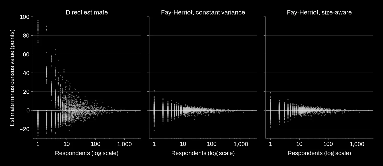
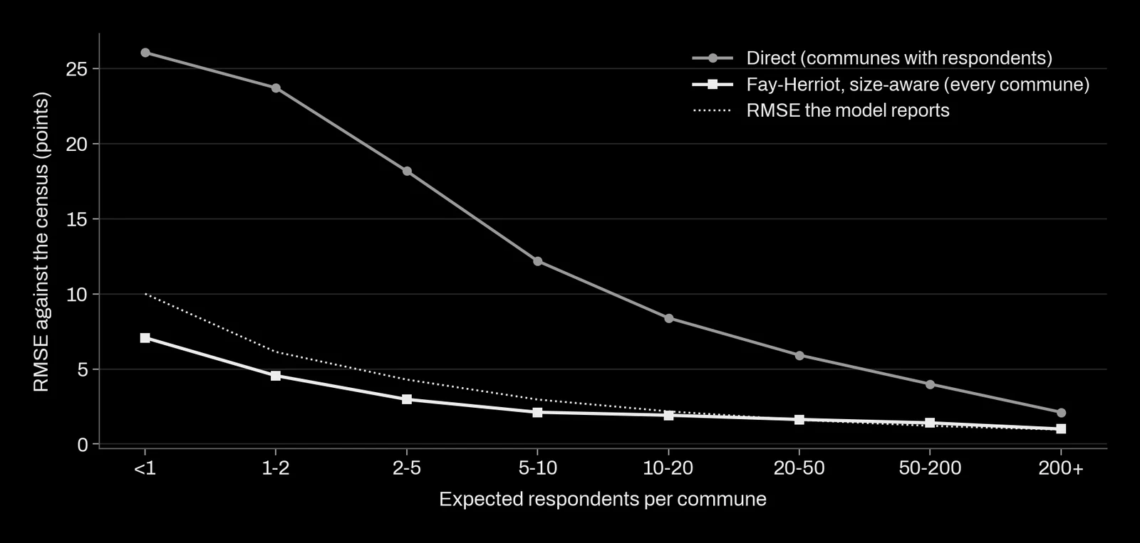
The gain is large and holds at every size. Among the 3,627 communes with a respondent in more than half of the surveys, the Fay-Herriot RMSE was lower than the direct RMSE in 99.6 % of them, and the typical commune's RMSE fell to 0.13 to 0.15 of the direct one depending on the variant, a drop of about 85 %. Even the 32 communes expecting 200 or more respondents saw their RMSE fall to about 0.4 of the direct one. By size, the size-aware variant described below had an RMSE of 4.6 points at 1 to 2 expected respondents (direct: 23.7), 3.0 points at 2 to 5 (direct: 18.2) and 1.9 points at 10 to 20 (direct: 8.4). In the surveys where a commune had no respondent, its estimate came from the regression alone, with an RMSE of 5.6 points.
Where the margins of error went wrong, and the fix
Our first version used the textbook recipe: each commune's sampling variance computed from the regional rate, ψi = p̄(1 − p̄)(1 − f)/ni, and a single area variance. Its estimates were good. Its 95 % intervals contained the census value in only 53.9 % of cases. In communes expecting 1 to 2 respondents, the model reported an RMSE of 1.1 points where the real one was 4.5. We found two causes.
The sampling variance was a little too large. Using the regional rate for every commune overstates the average sampling variance by the variance of the true rates across communes. That is a small amount, but with one to five respondents it is of the same size as σv² itself, and REML absorbs it by shrinking σv to 0.0093. Computing ψi from a smoothed rate instead (a weighted regression of the direct estimates on the auxiliary variables) raised σv to 0.0142 and coverage to 69.0 %.
Small communes vary more around the regression. The model assumes one area variance for all communes. In the census, the spread of the true rate around the regression is 5.0 points for communes under 100 active residents, 2.5 points from 100 to 500, 2.0 from 500 to 5,000 and 1.6 above. In a commune of 50 active residents, two people changing status move the rate by four points; that is variation in the truth, not in the survey. We let the area variance depend on size: σa² + σb² · p̄(1 − p̄)/Ni, where Ni is the number of active residents in 2017, known before the survey. REML estimated a floor of 0.0087 and a size coefficient of 2.39. The mean squared error formula extends to two variance parameters without change of principle.
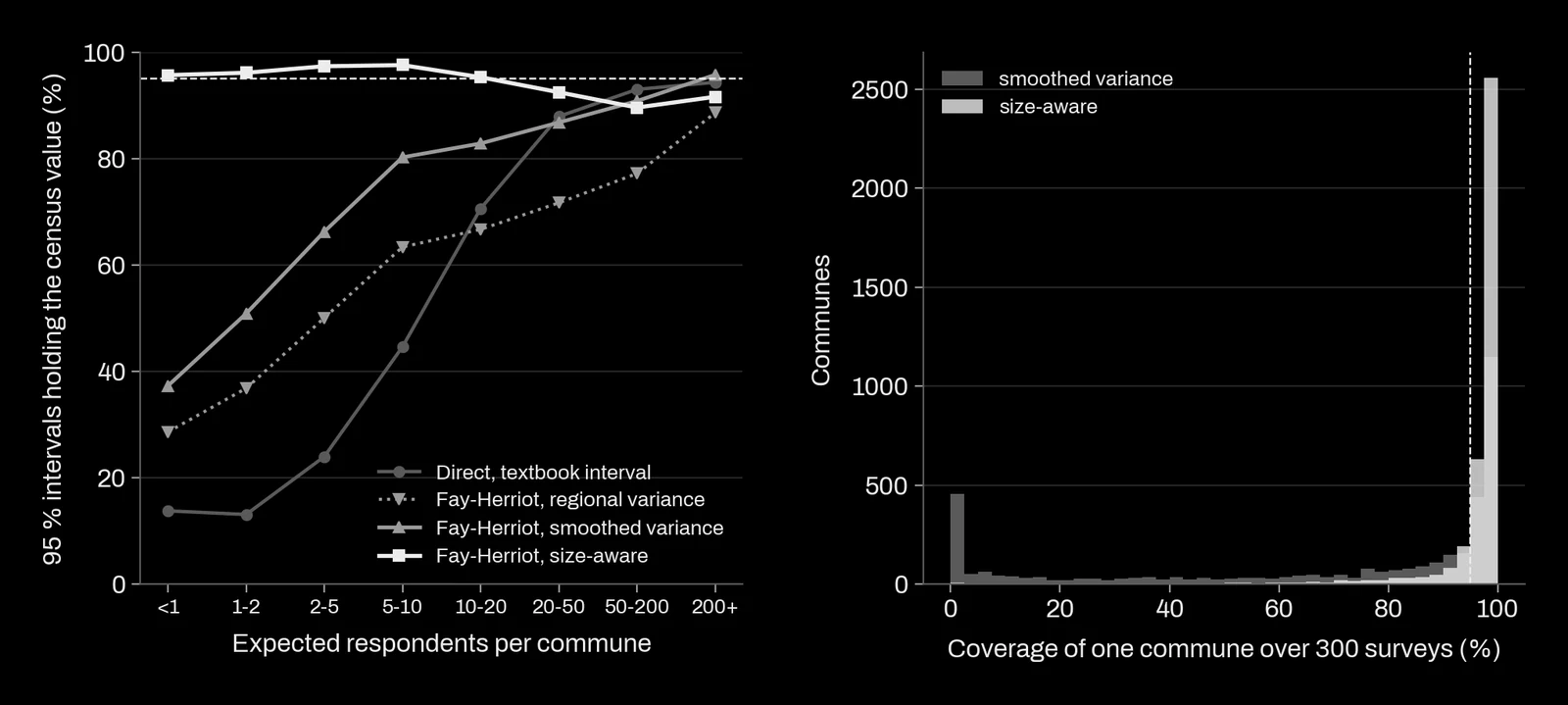
With both corrections, coverage was 96.1 % overall and between 89.6 % and 97.6 % in every size group. The share of communes whose own coverage fell under 85 % went from 44.6 % with the smoothed constant-variance model to 6.2 %. The price was a mean squared error 7.2 % higher across all communes (interval 5.9 % to 8.6 %), because the size-aware model trusts the regression less for small communes, and wider margins where they belong.
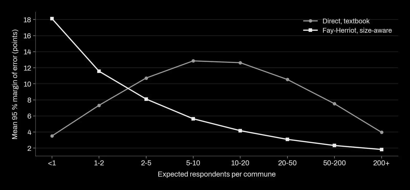
The honest margins are wide for small communes: about ±18 points for communes expecting fewer than one respondent, ±11.6 at 1 to 2, ±8.1 at 2 to 5, ±4.2 at 10 to 20 and ±1.8 for the largest. In the smallest group the reported RMSE (10.0 points) was above the real one (7.1), so those intervals are conservative; for commune surveys with no respondent at all, coverage was 96.2 %. One limit remains: coverage is an average over communes. For the 10 % of communes whose true rate is farthest from the regression, the size-aware intervals covered 82.8 % of the time, and the constant-variance ones 1.5 %. A model-based margin is correct on average across areas; for an atypical area it can be too narrow, and the analyst should know which areas those are likely to be.
How to do it on your own data
- Choose auxiliary variables that exist for every area and date from before the survey: an earlier census, a register, an administrative count. Check how well they predict the indicator where the survey is large.
- Compute sampling variances from a smoothed rate, not from each area's own estimate and not from one regional rate. With a complex design, include the design effect.
- Look at the spread of the direct estimates around the regression by area size. If small areas spread more than their sampling variance explains, let the area variance depend on size.
- Before publishing, simulate surveys from a known truth (a census, a register, or the fitted model itself) and measure RMSE and coverage by area size, as we did here.
- Publish each estimate with its margin and its weight on the direct estimate, and flag areas whose direct value is far from the model's prediction.
Limits of this example: simple random sampling of individuals, where real surveys sample households in clusters and have larger sampling variances; one region; a census value that for large communes is itself estimated from a sample; a model on the rate itself, where a transformation of the proportion is sometimes preferred; and no benchmarking, the step that makes area estimates add up to the published regional figure. Each of these changes the numbers, not the method of checking them.
What this means for a project
When we produce small area figures for a public body, you receive:
- an estimate for every area, including those with no respondent, with the share that comes from the survey and the share from the model;
- a margin of error per area, and a simulation that measures how often those margins contain the truth, by area size, before anything is published;
- the auxiliary data used, with their source, date and licence, and how well they predict the indicator;
- a list of the areas where the survey and the model disagree, so that a local expert can look at them.
What we will not do: publish a commune figure from five respondents without a model, publish model-based margins whose coverage we have not measured, or present a synthetic estimate as if it had been observed.
References
- Fay, R. E. and Herriot, R. A. (1979). Estimates of income for small places: an application of James-Stein procedures to census data. Journal of the American Statistical Association 74(366). doi:10.1080/01621459.1979.10482505
- Prasad, N. G. N. and Rao, J. N. K. (1990). The estimation of the mean squared error of small-area estimators. Journal of the American Statistical Association 85(409). doi:10.1080/01621459.1990.10475320
- Datta, G. S. and Lahiri, P. (2000). A unified measure of uncertainty of estimated best linear unbiased predictors in small area estimation problems. Statistica Sinica 10(2). openalex:W2186317843
- Rao, J. N. K. and Molina, I. (2015). Small area estimation, second edition. Wiley. doi:10.1002/9781118735855
- Ghosh, M. and Rao, J. N. K. (1994). Small area estimation: an appraisal. Statistical Science 9(1). doi:10.1214/ss/1177010647
- Pfeffermann, D. (2013). New important developments in small area estimation. Statistical Science 28(1). doi:10.1214/12-sts395