Model validation: placebo, positive control, sealed holdout

Why gates

A research team can fool itself in two directions. It can keep a result that is only noise, or throw away a real effect because its test could not see it. Both cost money: the first ships a model that fails, the second abandons one that would have worked. Our gates are built to make both errors visible, and to say which one a verdict is exposed to.

Every study goes through the same stages. Before any number, a written plan: the question, the mechanism we expect, the test, the thresholds and the sealed sample, frozen with a hash. Then development, where we may try as many things as we like, judged by three checks together. Then one read of the sealed sample. Finally an entry in an append-only evidence ledger.

Development: paired gain, placebo, planted effect

Paired gain. A candidate is compared to the reference on the same cases, case by case, and we report the mean difference with its interval. Comparing two summary figures is not the same thing. In one study a change looked worth +0.24 because the two arms had not been run on the same set of simulated programmes; on the same programmes it was worth +0.021.

Placebo. We give the method a version of the input with the information destroyed (shuffled labels, shifted dates, random alarms at the same frequency) and check that the result disappears. If the placebo does as well as the real thing, the gain comes from the mechanics of the method, not from the signal. A placebo must also be able to move something: we once ran one that produced 0 changes out of 1,078 decisions and read it as “the gate is sound”. It could not have failed.

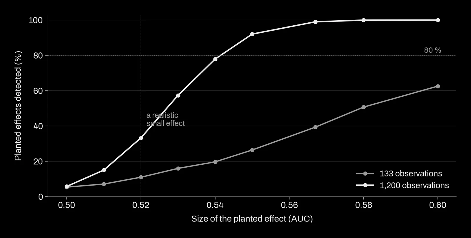
Planted effect, at several sizes. This is our positive control: we add a known effect to real data and check that the pipeline finds it. One size is not enough. In July 2026 a screen of options data planted an effect of information coefficient 0.10, large enough to trade, and the pipeline returned +0.007 with t = -0.02. With 1,229 days, twice the standard error of an information coefficient is about 0.057, while realistic effects in that domain are 0.02 to 0.04: the test could not see them. On a longer target (3,667 days) the bar fell to 0.033. On a narrow table, a regularised linear model detected the planted effect about twice as well as gradient-boosted trees (t = 3.85 against 1.91).

From several sizes we compute the detection floor: planted size times the judge's bar, divided by what was recovered. One harness for single stocks recovered 0.1218 from a planted 0.10 against a bar of 0.2961, a floor near 0.24, about eight times the effects the literature reports. Every “nothing found” it had produced meant nothing. The same design on a panel of 1.7 million rows and 499 names had a floor of 0.001.

Line chart of the share of planted effects detected against effect size, for 133 and 1,200 observations. At an AUC of 0.52, 11 percent are detected with 133 observations and 33 percent with 1,200; at 0.55, 26 and 92 percent. — Figure 1. Simulation. A binary outcome and one score with a planted effect of the size on the horizontal axis (binormal model), one-sided test of the AUC at 5 %, 3,000 replications per point. With 133 observations, an effect of 0.52 is found 11 % of the time and one of 0.567 39 % of the time; with 1,200 observations, 33 % and 99 %.

Three verdicts, not two

A test that finds nothing has two possible meanings. Either there is nothing to find, or the instrument is too weak. The planted effect tells them apart, so we use three verdicts:

Positive: paired gain with an interval above zero, placebo dead, planted effect recovered.
Negative: the planted effect is recovered at the size that would matter, and the real gain is not there. We state the size ruled out: “no effect of 0.03 or more”, never “no effect”.
Empty: the planted effect is not recovered at that size. The question is still open, and we say what sample size would close it.

An example from October 2026: a panel test of 368 rows gave a paired gain of -0.0095, interval -0.074 to +0.048, and the planted effect was found at only the largest of three sizes. That is empty, not negative. Reading it as negative would have closed a question the data never answered.

The resolution of a judge

Every judge has a resolution, the smallest difference it can tell from noise, and we measure it before using it. For the strategy evaluation, the pass rate was known to +/- 0.20 as a level, because the history held about 5.8 independent windows. A paired difference between two systems on the same windows was known to +/- 0.065. A single year alone, to +/- 0.53.

These numbers gave us our most instructive bug. One gate required that no single year lose more than a set amount. On 2 August we found it used the global paired resolution, 0.065, for one year. A year weighs about one window, not 5.8, so the gate was about 2.4 times too severe and was rejecting good candidates. We set it to 0.065 times the square root of 5.8, 0.157.

Then a note appeared saying the number of independent windows was really 11.3, so the gate should be 0.218. Before paying that debt we reread the derivation already in our code: the number of windows cancels out. The spread of one year relative to the whole is the square root of the number of years in the data. The 0.157 had been right by coincidence, because 5.8 windows happened to sit close to 5.6 years on that feed. The “fix” would have made the gate 42 % too lax on that feed.

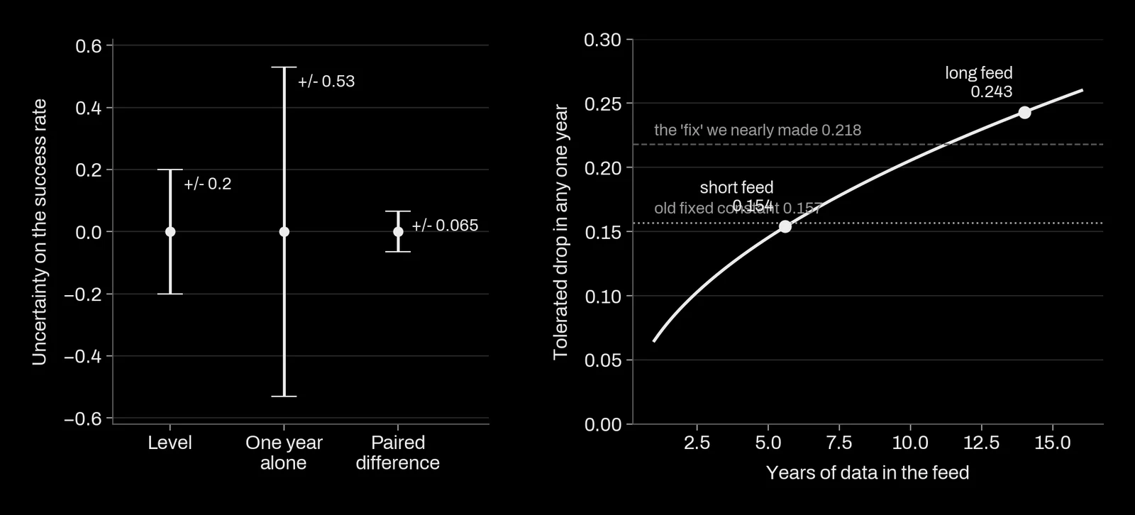
Left: three error bars, +/- 0.2 for a level, +/- 0.53 for one year alone, +/- 0.065 for a paired difference. Right: curve of tolerated drop in one year against years of data, 0.065 times the square root of years, with the short feed at 0.154 and the long feed at 0.243, and horizontal lines at the old constant 0.157 and the near-fix 0.218. — Figure 2. Real values. Left: resolution of the pass-rate judge. Right: the annual gate as a function of the years in the feed, 0.065 times the square root of years. It is 0.154 on the feed starting in 2021 (the old constant was 2 % off) and 0.243 on the feed starting in 2012, where the old constant was far too tight.

We removed the constant and now compute the gate from the span of each feed. The rule we keep: a constant that is right by coincidence is a bug waiting for its next dataset. The fix is never a new value; it is to compute the quantity the constant stood for.

One read of a sealed sample

Development is free: we try what we want, and we report how many things we tried. The protection against fooling ourselves is the sealed sample. It is set aside in the plan, locked in code (the loader refuses its dates unless a flag is set), and read once, by a script that takes the sample's hash and refuses a second read. A single read of a single frozen candidate has no multiple-testing problem, so it is judged at the nominal threshold.

A sealed sample can burn without being opened. In October 2026 an independent review of our code found that the years of one sealed sample had already been used by another bench, and that the label of a second was public at prediction time in 43 % of cases. Both were declared burned and the readers now refuse them. One question became unconfirmable until fresh data exists, and its replacement is a prospective sample that cannot be read before September 2028. We would rather wait than confirm on a sample that was already seen.

An evidence ledger instead of a pass mark

A pass mark throws away small real effects: a result just under the bar is recorded as nothing. We record evidence instead, as e-values (Vovk and Wang 2021; Shafer 2021; Grünwald, de Heide and Koolen 2024). An e-value above 1 is evidence for an effect, below 1 against. Two properties make it the right tool for a research log. The weighted average of e-values stays an e-value however dependent they are, so correlated markets or models can be merged without a model of the correlation. And evidence from fresh data multiplies, and stays valid whether we stop or continue, so a small positive has a path instead of dying at its first test.

The ledger (append-only) turns each p-value into an e-value with a fixed calibrator, e = 0.5 p^-0.5. It refuses to multiply evidence from data it has already seen. It takes whole campaigns, never only their survivors, because a ledger fed with winners hides the winner's curse where nobody looks.

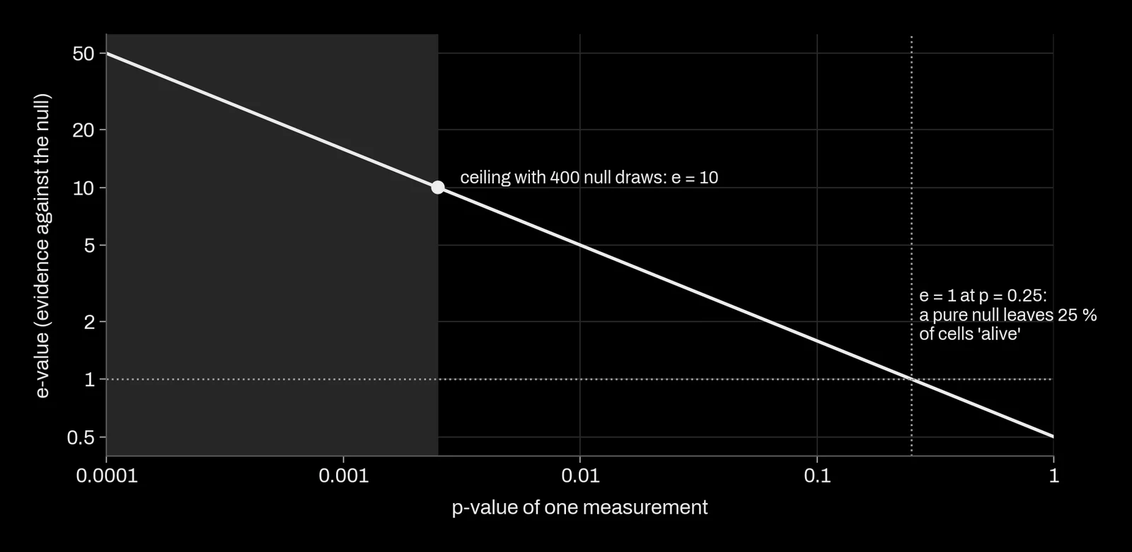
Log-log line chart of e-value against p-value: e equals 1 at p = 0.25 and 10 at p = 1/401, the smallest p-value available with 400 null draws. — Figure 3. The calibrator used by the ledger, e = 0.5 p<sup>-0.5</sup>. Two facts we print with every entry: under pure noise a quarter of cells reach e of 1 or more, so the count expected by chance is always shown next to the count observed; and with 400 null draws the smallest possible p-value caps the evidence of one measurement at e = 10.

Building it, we hit the obvious trap: a Monte Carlo p-value of exactly 0 is not infinite evidence, it is the resolution of the null. Without the usual +1 correction the merged evidence of one campaign came out at 42,931. Refilling the ledger with 571 past cells, without re-measuring anything, showed one family of commodity signals below chance (92 cells at e of 1 or more where 114 were expected), so empty. A cluster we first took for a coherent family was at chance too; its high values were maxima of 30 draws.

Laws that run

Over two days in late July we wrote down eight lessons from eight bugs. The eighth bug had the same shape as the first. Writing a lesson down had prevented nothing. All eight shared a pattern: a component ran, returned a clean output, and the output meant nothing because some property of its input had not been checked.

Since then the lessons are code. A preflight module runs before any verdict and raises an error, not a warning, if a check fails. Among the checks: features really distinct after the transformation actually used; the effective number of independent units; a null statistic with enough distinct values; a control that can both fail and pass; a sign convention checked against a known value; no ratio with a denominator near zero. Replayed against the eight old bugs, it caught 9 of 9 defects before any verdict. On its first real run it found two we had missed: our own effective-sample-size function returned 0 on a matrix with gaps, and one null had only 3 distinct values over 400 draws, which voided every p-value on that corpus.

A component that returns a verdict calls the preflight. If it does not, it may not conclude. When a bug teaches us something, the question is no longer where to write it down but which assertion would have caught it.

What this means for a project

For each question in your project, you receive:

the plan as written before the results, with its date and hash;
the paired gain against your current method or a simple benchmark, with its interval, the placebo and the planted-effect test;
a verdict of positive, negative or empty, and for an empty verdict the amount of data that would settle it;
the result of one read of a sample kept aside from the start, and the number of things tried before it.

What we refuse to claim: that nothing works when our test could not have seen it, a difference smaller than the judge's resolution, or a confirmation on a sample we had already looked at.

References

Vovk, V. and Wang, R. (2021). E-values: calibration, combination and applications. The Annals of Statistics 49(3). doi:10.1214/20-AOS2020
Shafer, G. (2021). Testing by betting: a strategy for statistical and scientific communication. Journal of the Royal Statistical Society A 184(2). doi:10.1111/rssa.12647
Grünwald, P., de Heide, R. and Koolen, W. (2024). Safe testing. Journal of the Royal Statistical Society B. doi:10.1093/jrsssb/qkae011
Ramdas, A., Grünwald, P., Vovk, V. and Shafer, G. (2023). Game-theoretic statistics and safe anytime-valid inference. Statistical Science 38(4). doi:10.1214/23-STS894
Harvey, C. R. and Liu, Y. (2020). False (and missed) discoveries in financial economics. The Journal of Finance 75(5). doi:10.1111/jofi.12951

Our gates: placebo, positive control and a sealed holdout