

What a validation report has to answer
A credit scoring model estimates the probability that a borrower will default. A validation report tells a lender, an auditor or a supervisor whether those probabilities can be used, for what, and with which limits. We built a model on public data, validated it the way we would validate a client's model, and kept every number the code printed.
The report answers six questions, in this order:
- Does it rank? On unseen data, and by how much more than a simple benchmark?
- Are the probabilities right? When the model says 20 %, do about 20 % default?
- Is the population stable? Does the scored data look like the development data?
- Does it work for every group? Results by segment.
- Could the result be an artefact? A placebo with shuffled labels must score at chance.
- What can it not tell us? The limits, written down.
The regulatory context explains why these questions have become formal. In the European Union, AI systems intended to evaluate the creditworthiness of natural persons or establish their credit score are listed as high-risk in Annex III, point 5(b) of the AI Act (Regulation (EU) 2024/1689), with an exception for systems used to detect financial fraud. The amending Regulation (EU) 2026/1744 moved the date from which the high-risk requirements apply to systems in Annex III from 2 August 2026 to 2 December 2027. For banks, the supervisory guidance on model risk known as SR 11-7, the reference most validation teams were built around, was superseded on 17 April 2026 by SR 26-2. We cite these texts for context only; what they require of a given lender is a legal question, not a statistical one.
The data and the split
We used the “Default of credit card clients” dataset of Yeh and Lien, published on the UCI Machine Learning Repository under a CC BY 4.0 licence. It holds 30,000 credit card clients of a bank in Taiwan, with their credit limit, age, sex, education, marital status, and six months of repayment status, bill amounts and payments from April to September 2005. The label is whether the client defaulted on the next payment. The default rate is 22.12 %.
A data audit comes before any model. No values are missing and no ID is duplicated, but three things would go into the report. Education carries 345 rows with codes 0, 5 and 6 that the documentation does not define, and marital status 54 rows with code 0; we merged them into “other”. More important, the documented scale of repayment status runs from −1 (paid duly) to 9 (nine months late), yet 58.3 % of clients have −2 or 0 in the latest month, two codes the documentation never explains. On a real portfolio we would ask the data owner; here we kept them as ordered values, an assumption we state.
The dataset has no application or observation dates, so an out-of-time test, the standard for credit models, is impossible. Only a test on later applications meets new products, a new cycle or a changed acceptance policy; a random split cannot. We drew a stratified random 30 % of clients (9,000) as a sealed holdout with a fixed seed, built and compared everything on the other 21,000 with five-fold cross-validation, and opened the holdout once, from one script, after every choice had been made. The time dimension of validation is the subject of our note on time series validation.
Sex and marital status were left out of the model inputs. They are kept in the data only to check the model by segment.
A benchmark, then the model
We fixed two models before looking at any result.
- Benchmark: a logistic regression on five variables a credit analyst would pick first: repayment status in the last two months, the log of the credit limit, utilisation (last bill divided by limit) and the share of the previous bill repaid.
- Model: gradient boosting on 41 inputs (the raw history plus utilisation and repayment ratios for each month and the worst delay over six months), with hyperparameters set once and not tuned: learning rate 0.05, 300 trees, 15 leaves, at least 50 clients per leaf.
In development, five-fold cross-validation gave an AUC of 0.707 for the benchmark (folds between 0.705 and 0.712) and 0.777 for boosting (0.773 to 0.783). Inside the benchmark, the standardised coefficient of the latest repayment status is 0.641, more than twice any other; the share of the previous bill repaid has a coefficient of zero at three decimals. The benchmark's job is to price the complexity of the model: a model that cannot beat five variables by more than its interval does not earn its maintenance cost. Large comparisons of credit scoring methods, such as Lessmann and co-authors (2015), find ensembles ahead of logistic regression on average across datasets, by margins that vary from one portfolio to the next.
Discrimination, with intervals
The AUC is the probability that a randomly chosen defaulter gets a higher score than a randomly chosen non-defaulter. The Gini coefficient used in credit is 2 × AUC − 1. We give each with a 95 % interval from 2,000 bootstrap resamples of the holdout, and compare the two models on the same resamples, because their errors are correlated and a paired difference is far more precise than two separate intervals.
| Measure | Logistic benchmark | Gradient boosting |
|---|---|---|
| AUC, development cross-validation | 0.707 | 0.777 |
| AUC, sealed holdout | 0.734 (0.722 to 0.747) | 0.794 (0.783 to 0.805) |
| Gini, sealed holdout | 0.469 (0.443 to 0.495) | 0.588 (0.565 to 0.610) |
| Defaults caught in the riskiest 10 % | 30.0 % | 31.5 % |
| Defaults caught in the riskiest 20 % | 50.7 % | 51.4 % |
| Brier score (base rate alone: 0.172) | 0.143 | 0.133 |
| Calibration slope / intercept | 1.144 / −0.011 | 0.996 / −0.022 |
| Hosmer-Lemeshow, 10 groups | 220.6 (p < 0.001) | 12.9 (p = 0.12) |
Boosting gains 0.060 of AUC over the benchmark, with a paired interval of +0.049 to +0.071; none of the 2,000 resamples showed a gain of zero or less. The gain is real. Its practical size is smaller than the AUC suggests: in the riskiest 20 % of clients, boosting catches 51.4 % of defaults against 50.7 % for the benchmark. Most of the extra ranking happens in the middle of the score range, which matters for pricing and limits more than for a single cut-off.
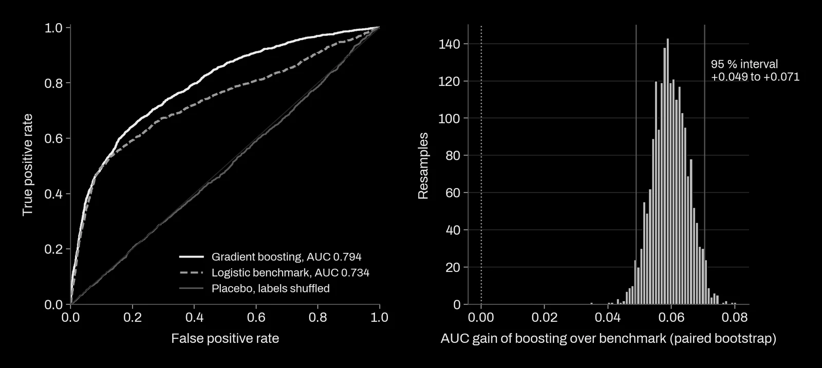
Two readings of this table need care. The first is overfitting: boosting scored 0.858 on its own training data and 0.794 on the holdout. Only the second number may be reported. The second is less obvious. Both models did better on the holdout than in development: the benchmark by 0.027 of AUC. After the single read, we checked whether our split was unusual by repeating the benchmark's development and holdout on 40 other random splits. The holdout-minus-development gap averaged −0.002 with a standard deviation of 0.010 and never exceeded +0.021. Our holdout is a lucky draw. The report says so and gives the development estimate of 0.777 as the better guide to the level to expect. The paired comparison between models does not carry this luck.
Calibration: are the probabilities right?
A score can rank well and still give wrong probabilities. If probabilities feed pricing, provisions or capital, calibration matters as much as ranking. We report four checks.
- Calibration in the large: the mean predicted rate against the observed rate. Benchmark 22.29 %, boosting 22.41 %, observed 22.12 %.
- Calibration slope and intercept (Cox, 1958): regress the outcome on the log-odds of the prediction. A slope below 1 means predictions are too extreme, above 1 too timid.
- Brier score: the mean squared error of the probability, compared to the score of predicting the base rate for everyone.
- Hosmer-Lemeshow: a chi-square test over ten score groups.
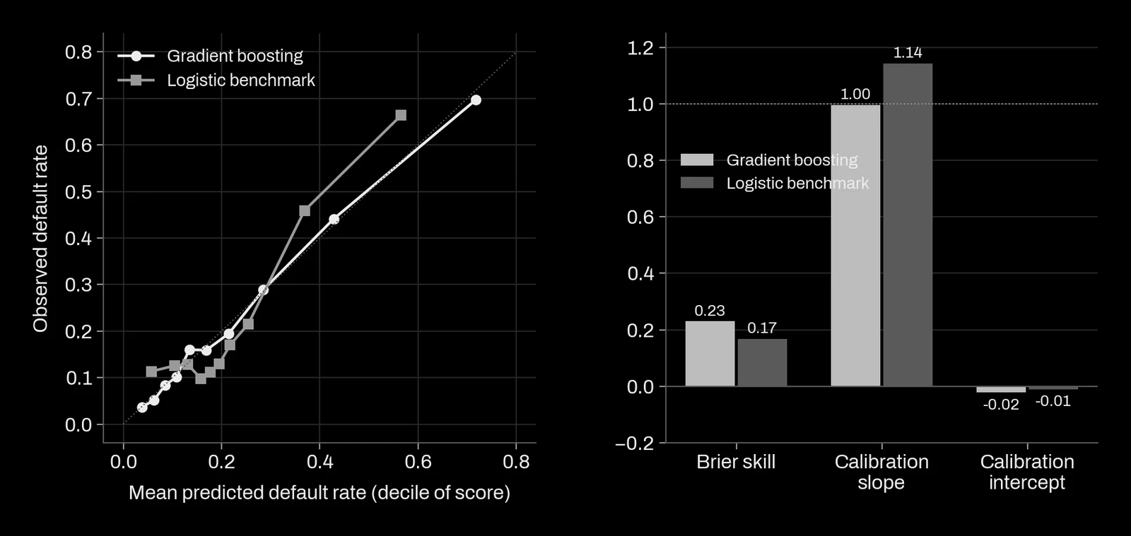
Boosting is close to perfect on this holdout: slope 0.996, intercept −0.022, a Brier skill of 0.23 over the base rate. The benchmark ranks reasonably but its probabilities are too compressed (slope 1.144): its riskiest decile is predicted at 56.5 % and observed at 66.3 %, its two safest deciles are predicted at 5.7 % and 10.4 % and observed at 11.3 % and 12.6 %, and its middle deciles are predicted too high. A lender pricing from it would undercharge the worst risks.
On the Hosmer-Lemeshow test, a word of caution. With 9,000 clients it rejects almost any small misfit, and with a few hundred it has little power to see a large one. Its p-value of 0.12 for boosting is reassuring here, but we read the reliability curve and the slope first; Van Calster and co-authors (2019) make the same recommendation. Calibration is also the first thing to break when the population moves, as the next section shows.
Stability: PSI and what it misses
The population stability index (PSI) compares the distribution of a score, or of an input, between two samples: bin the development values into deciles, then sum (share in new − share in development) × ln(share in new / share in development) over the bins. The usual thresholds of 0.1 and 0.25 are conventions; Yurdakul and Naranjo (2020) work out the sampling distribution of the index, which depends on the sample sizes and the number of bins, so a fixed threshold means different things on 2,000 and on 200,000 accounts.
Between development and holdout, the score PSI is 0.002 and the input PSIs are all at or below 0.002 (limit 0.001, age 0.001, utilisation 0.002, last repayment status 0.0004). That is what a random split must give, so on its own it proves nothing. To show what the check is for, we redrew the holdout as a different book: clients under 30 three times as likely to be drawn, and clients with a limit above the development median half as likely. The share of clients under 30 went from 32.3 % to 62.0 %.
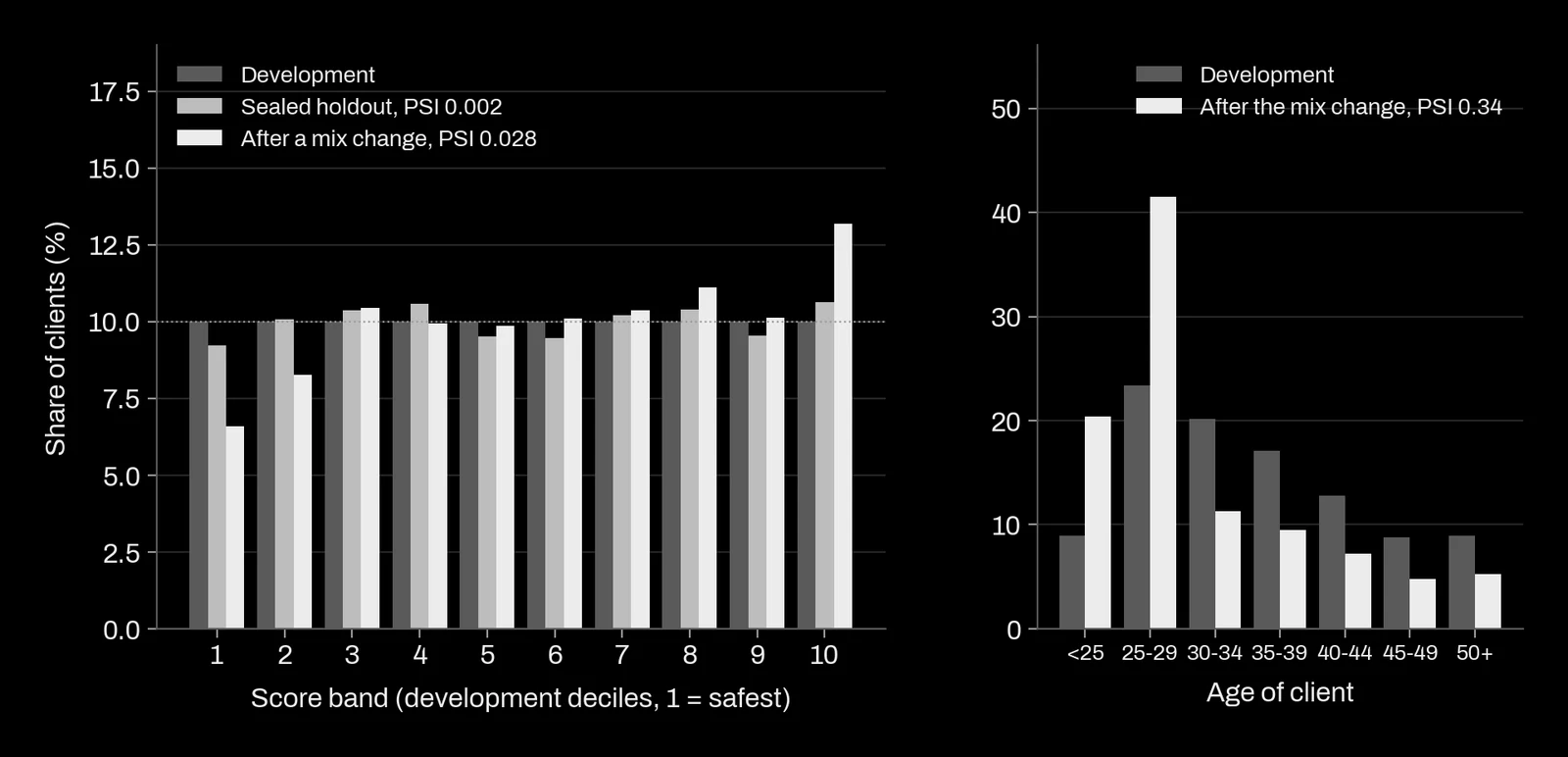
The age PSI jumped to 0.34, far over any threshold. The score PSI only reached 0.028, well under the 0.1 that would trigger a review. On that shifted book, AUC stayed at 0.787, but the observed default rate was 25.3 % against 24.5 % predicted, and the calibration intercept moved from −0.022 to +0.051. A monitoring plan that tracks only score PSI would have missed it. We monitor input PSIs and calibration in the large together, on every scoring batch.
Discrimination by segment
An overall AUC can hide a group where the model is weak. We computed it by segment, with observed and predicted default rates.
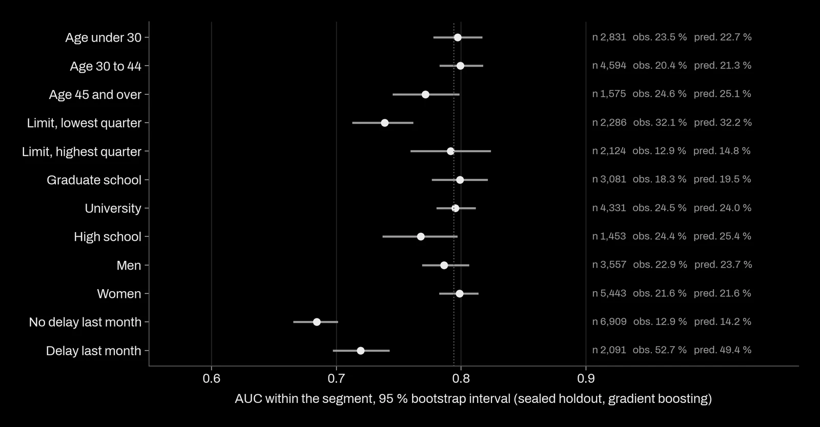
Three findings would go into the report. First, the model ranks less well inside the lowest limit quarter (0.739, interval 0.713 to 0.761), where the default rate is 32.1 %; calibration there is good (32.2 % predicted). Second, the overall AUC owes a lot to one variable: among clients with no delay last month, AUC falls to 0.684, and among those with a delay to 0.720. Within each group the model is a weaker tool than its headline says. Third, calibration drifts at the edges: the model predicts 14.8 % for the highest limits where 12.9 % default, and 49.4 % for recent delays where 52.7 % default.
By sex, which the model does not use, AUC is 0.786 for men and 0.799 for women with overlapping intervals, and predicted rates are within 0.8 points of observed rates for both. This is a first check, not a fairness audit: inputs such as limit and education can carry information about protected attributes, and what counts as unfair treatment is set by law and by the lender's policy, not by an AUC.
The placebo: can the pipeline find signal in noise?
We trained the boosting model 20 times on the development data with the labels shuffled, then scored the real holdout labels. If the pipeline leaked information, through an identifier correlated with the label, a feature built with the outcome, or a preprocessing step fitted on all data, a shuffled model could still score above chance. It did not: mean AUC 0.496, range 0.457 to 0.526. That range is what chance alone produces on 9,000 clients.
A placebo cannot catch a leak present in both samples, such as a variable recorded after the default; that needs a check of when each input was known, covered in how we treat data.
What a validator should ask for
If you receive a validation report for a credit model, these are the questions we would ask, and that our own reports answer:
- Was the test sample out of time? If not, why not, and what does the report say about it?
- Was the test sample opened once, after every choice? Who held it?
- What is the benchmark, and what is the paired gain over it with an interval?
- Are AUC and Gini given with intervals?
- What do the calibration slope and intercept say, beyond a Hosmer-Lemeshow p-value?
- What are the PSIs of the inputs, not only of the score?
- How does the model perform by segment, including segments it does not use as inputs?
- What did a placebo score?
- How many models and settings were tried before this one? Our note on detecting overfitting explains why this count matters.
What this means for a project
On a credit scoring or model validation project with us, you receive:
- a data audit: undocumented codes, coverage, dates, with every assumption written down;
- a benchmark built before the model, and the paired gain of the model over it with an interval;
- a sealed test, out of time when the data has dates, opened once by a script;
- discrimination, calibration, stability and segment results as in this note, with the code that produced them;
- a placebo run and its result;
- a monitoring plan: input and score PSIs and calibration in the large, computed on every scoring batch, with alert levels set for your volumes.
What we refuse to claim: a holdout level as the level you will see next year, an in-sample AUC, or a fairness verdict from one table. The script behind every number on this page is kept with the site sources and reruns with the same seeds.
References
- Yeh, I.-C. (2009). Default of credit card clients [dataset]. UCI Machine Learning Repository, licence CC BY 4.0. doi:10.24432/C55S3H
- Yeh, I.-C. and Lien, C.-H. (2009). The comparisons of data mining techniques for the predictive accuracy of probability of default of credit card clients. Expert Systems with Applications 36(2). doi:10.1016/j.eswa.2007.12.020
- Hanley, J. A. and McNeil, B. J. (1982). The meaning and use of the area under a receiver operating characteristic (ROC) curve. Radiology 143(1). doi:10.1148/radiology.143.1.7063747
- Efron, B. (1979). Bootstrap methods: another look at the jackknife. The Annals of Statistics 7(1). doi:10.1214/aos/1176344552
- Cox, D. R. (1958). Two further applications of a model for binary regression. Biometrika 45(3-4). doi:10.1093/biomet/45.3-4.562
- Brier, G. W. (1950). Verification of forecasts expressed in terms of probability. Monthly Weather Review 78(1). doi:10.1175/1520-0493(1950)078<0001:VOFEIT>2.0.CO;2
- Hosmer, D. W. and Lemeshow, S. (1980). Goodness of fit tests for the multiple logistic regression model. Communications in Statistics, Theory and Methods 9(10). doi:10.1080/03610928008827941
- Van Calster, B., McLernon, D. J., van Smeden, M., Wynants, L. and Steyerberg, E. W. (2019). Calibration: the Achilles heel of predictive analytics. BMC Medicine 17. doi:10.1186/s12916-019-1466-7
- Yurdakul, B. and Naranjo, J. D. (2020). Statistical properties of the population stability index. The Journal of Risk Model Validation. doi:10.21314/jrmv.2020.227
- Lessmann, S., Baesens, B., Seow, H.-V. and Thomas, L. C. (2015). Benchmarking state-of-the-art classification algorithms for credit scoring: an update of research. European Journal of Operational Research 247(1). doi:10.1016/j.ejor.2015.05.030
- Friedman, J. H. (2001). Greedy function approximation: a gradient boosting machine. The Annals of Statistics 29(5). doi:10.1214/aos/1013203451
- Regulation (EU) 2024/1689 (Artificial Intelligence Act), Annex III, point 5(b). eur-lex.europa.eu/eli/reg/2024/1689
- Regulation (EU) 2026/1744 of 8 July 2026 (Digital Omnibus on AI), amending Article 113 of Regulation (EU) 2024/1689. eur-lex.europa.eu/eli/reg/2026/1744
- Board of Governors of the Federal Reserve System (2026). SR 26-2, Revised Guidance on Model Risk Management, 17 April 2026, superseding SR 11-7. federalreserve.gov/supervisionreg/srletters/SR2602.htm